Fundamentals

Fringes is an easy to use, pure-python tool. It provides the key functionality which is required in both, fringe projection [1] and deflectometry [2]: positional coding by virtue of phase shifting.

“Of particular importance in the analysis and design of communication systems are the characteristics of the physical channels through which the information is transmitted” [3]. The channel, i.e. the used hardware (camera, test object, screen), cause the following transmission impairments:

• attenuation,

• blurring,

• noise.

The reason for coding is efficient and reliable information transmission. Here, information is the position where each camera sight ray is looking onto the screen. The screen pixel coordinte \(x\) is encoded via discrete gray values, the so-called phase shifting sequence \(I\).

In the following, the coding is considered for the horizontal direction only. The procedure is analogous in the vertical direction. For easier readibility, we drop the spatial and temporal dependencies of the quantities whenever practicable, i.e. we write \(I\) instead of \(I(x, t)\).

Encoding

1. Spatial Modulation

   The pixel coordinate \(x\) of the screen is normalized into the range \([0, 1)\) by dividing through the screen length \(L\) and used to spatially modulate the radiance \(I\) in a sinusoidal fringe pattern

   \(I = a + b \cos(\varPhi) = a + b \cos(2 \pi \nu_i x / L - \varphi_0)\)

   with offset \(a\), amplitude \(b\), global phase \(\varPhi\) and spatial frequency \(\nu\). An additional phase offset \(\varphi_0\) may be set, e.g., to let the fringe pattern start with an arbitrary value \(\in [0,I_{max}]\) with \(I_{max} = a + b\). There can be \(K\) fringe patterns, each with different spatial frequency \(\nu_i\), with \(i \in \{ \, \mathbb{N}_0 \mid i < K \, \}\).

2. Temporal Modulation

   \(I = a + b \cos(2 \pi \nu_i x / L - 2 \pi f_i t_{i,n} - \varphi_0)\)

   The fringe patterns of each set \(i\) are then modulated temporally, i.e. shifted \(N_i\) times with an equidistant phase shift of \(2 \pi f_i / N_i\). This is equal to sampling over \(f_i\) periods with \(N_i\) sample points at time steps \(t_{i,n} = n / N_i\), with \(n \in \{ \, \mathbb{N}_0 \mid n < N_i \, \}\).

Transmission

The transmission channel consists of the following components with their associated effects:

• screen (light source): photon shot noise

• surrounding: ambient light sources (increasing \(a\))

• test oject: distortion (deflection), absorption (decreasing \(a\)), scattering (decreasing \(b\))

• camera lens: defocus / blurring (decreasing \(b\))

• camera: electronic shot noise, temporal dark noise, quantization noise

Combined, this results in the following main effects:

1. Distortion

   The camera sight ray originating from the camera pixel \(x_c\) gets deflected by the test object onto a screen coordinate \(x\). Depending on the object shape and slope, the spatial alignment of the fringe pattern \(I\) is altered. For specular surfaces, the test object basically becomes part of the imaging optics.

1. Blurring

   The camera sight ray is modeled as an infitesimal thin ray in space, sampling the test object and finally arriving on the illuminating fringe pattern \(I\). Its reflection off (transmission through) an object results in a scattering lobe (cf. Fig. 1). The intersection of the scattering lobe with the screen surface is the so-called point spread function (PSF).

   

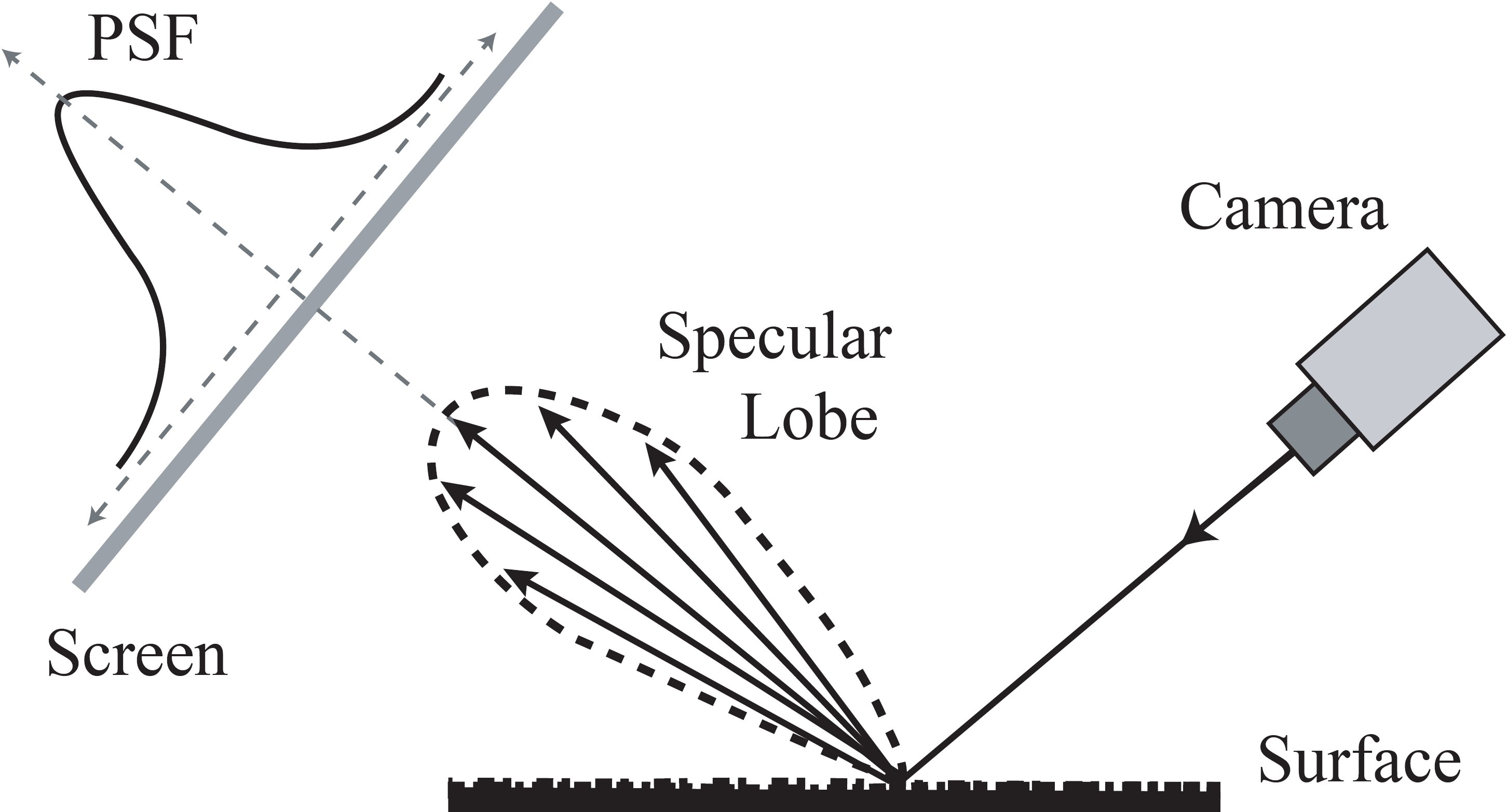
   Fig. 1 Projecting the scattering lobe of the surface onto the screen results in a point spread function (PSF). From [4].

   We assume the transmission system to be a linear, shift invariant system \(\mathcal{L}\{ \cdot \}\). The PSF is the spatial impuls response \(h\) of the system, blurring the original fringe pattern \(I\):

   \(I'(x) = I(x) * h(x)\)

   where \(*\) denotes the convolution operator.

   The modulation transfer function \(MTF\) is the normalized magnitude of the Fourier-transformed PSF; \(b'\) denotes the measured modulation.

   \(MTF(\nu) = | \mathcal{F}\{h(x)\} | = H(\nu) = \frac{b'(\nu)}{b(\nu)} \le 1\)

   The \(MTF\) indicates how well a structure with spatial frequency \(\nu\) is transmitted by an optical system. More precisely: it indicates how well the amplitude of a sinusoidal object is retained in the image, cf. Fig. 2.

   

   Fig. 2 Modulation transfer function (MTF) of an ideal optical system with circular aperture, depending on the spatial frequency \(\nu\) and the cut-off frequency \(\nu_c\).

1. Temporal noise

   We assume a linear sensor, i.e. the digital signal increases linearly with the number of photons received. We further assume the parameters describing the noise to be invariant with respect to time and space, i.e. the temporal noise at one camera pixel is statistically independent from the noise at all other pixels and the temporal noise in one image is statistically independent from the noise in the next image. All this implies that the power spectrum of the noise is flat both in time and space assuming white noise. These assumptions describe the properties of an ideal camera or sensor as described by the EMVA Standard 1288 [5].

   The following noise types are present:

   • photon noise (Poisson distributed)

   • elecronic noise (Poisson distributed)

   • dark noise (normally distributed)

   • quantization noise (equally distributed)

   Usually the central limit theorem applies, so we can model them as one normally distributed noise process. Hence, we model the measured irradiance readings \(I^*\) as superimposed with additive white Gaussian noise (AWGN) \(n(t)\):

   \(I^*(x, t) = I'(x) + n(t)\)

Decoding

1. Temporal Demodulation

   From the transmitted phase shifting sequence \(I^*\) we compute for each set i the average \(\hat{a_i} = \frac{\sum_n I^*_{i,n}}{N_i}\) (the indices \(i,n\) represent the shifts \(n\) per set \(i\)). It should be identical for all sets, so we can average all \(\hat{a_i}\) or simply average all \(I^*\). This yields the offset (also called brightness)

   \(\hat{a} = \frac{\sum_i \hat{a_i}}{K} = \bar{I^*}\).

   Then, we compute the temporal sampling points of the phase shifting on the unit circle in the complex plane \(c_{i, n} = e^{\mathrm{j}(2 \pi f_i t_{i,n} + \varphi_0)}\) and build up the complex phasor \(z_i = \sum_n I^*_{i,n} c_{i,n}\) with the measured irradiance readings \(I^*_{i,n}\) as the weights for the sampling points \(c_{i,n}\).

   From the complex phasor, we compute the modulation (average signal amplitude)

   \(\hat{b_i} = |z_i| \frac{2}{N_i}\).

   The factor 2 is because we also have to take the amplitudes of the frequencies with opposite sign into account.

   The argument of the complex phasor \(z_i\) is the circular mean of the irradiance-weighted sample points \(c_{i, n}\) and yields the phase map

   \(\hat{\varphi_i} = \arg(z_i) \mod 2 \pi\).

   The modulo operation maps the result of the arctan2-function from the range \([-\pi, \pi]\) to \([0, 2\pi)\). Due to the nature of the trigonometric function used, the global phase \(\varPhi = 2 \pi \nu_i x - \varphi_0\) is wrapped into the interval \([0, 2 \pi)\) with \(\nu_i\) periods.

   Tip

   For more details, e.g. on how to tailor your own custom phase-shifting formulae exactly adapted for your specific measurement task, please refer to [6].

2. Spatial Demodulation (Phase Unwrapping)

   To obtain the encoded coordinate \(x\), three tasks must be executed:

   i Undo the spatial modulation

   by finding the correct period order number \(k_i \in \{ \, \mathbb{N}_0 \mid k_i < \lceil \nu_i \rceil \, \}\) for each set \(i\), where \(\lceil \cdot \rceil\) denotes the ceiling function. The global phase maps are then estimated to be

   \(\hat{\varPhi_i} = \hat{\varphi_i} + k_i 2 \pi\).

   ii Recover the common independent variable

   by linearly rescaling each global phase map:

   \(\hat{x_i} = \frac{\hat{\varPhi_i}}{2 \pi} \lambda_i\)

   with \(\lambda_i\) being the spatial wavelength of the fringes (in pixels).

   iii Fuse the \(K\) coordinate maps

   by weighted averaging:

   \(\hat{x} = \frac{\sum_i w_i \hat{x_i}}{\sum_i w_i}\)

   To obtain an optimal estimate, use inverse variance weighting, i.e. use the precision (the reciprocal of the variance) of the coordinate maps as the weights for averaging:

   \(w_i = \frac{1}{\sigma_{\hat{x_i}}^2} \propto N_i \hat{b_i}^2 {\nu_i}^2\) [7].

   Depending on the coding parameterization, one of the following unwrapping methods is deployed:

1. No Unwrapping

   If only one set \(K = 1\) with spatial frequency \(\nu \le 1\) is used, no unwrapping is required, because one period covers the complete coding range. In this case, only the scaling part (ii) has to be executed.

2. Temporal Phase Unwrapping (TPU)

   If multiple sets, i.e. \(K \le 2\), with different spatial frequencies \(\nu_i\) are used, and the unambiguous measurement range is larger than or equal to the screen length, i.e. \(UMR \ge L\), the ambiguity of the phase map is resolved by generalized multi-frequency temporal phase unwrapping (GTPU).

3. Spatial Phase Unwrapping (SPU)

   However, if only one set with \(\nu > 1\) is used, or multiple sets but \(UMR < L\), the ambiguous phase \(\varphi\) is unwrapped by analyzing phase values in the spatial neighborhood [8]^, [9].

   Warning

   This only yields a relative phase map, therefore absolute positions remain unknown.

Tip

For a deeper study of fringe pattern analysis, please refer to [10].

Summary

Now we can state how the transmission impairments are adressed by the phase shifting coding scheme:

• Attenuation and Noise:

  Temporal demodulation is a matched filter (digital lock-in amplifier), selective to the temporal frequency \(f_i\). Therefore, even when the (attenuated) signal is close to the noise level in the time domain, they can be separated sufficiently in the frequency domain. It is optimally in the least-squares sense and hence is a maximum likelihood estimator in the presence of AWGN (additive white Gaussian noise).

  Also, fusing the coordinate maps using inverse variance weighting acts as the maximum lokelihood estimate \(\hat{x}\) for the true value \(x\).

• Blurring:

  Sinusoidal fringe patterns have the advantage over binary ones in that they are are Eigenfunctions of the optical system, i.e. they have no higher harmonics and therefore remain unchanged even for blurred imaging. Although their modulation \(b\) is attenuated, the desired coordinate \(x\) is determined with sub-pixel precision [11].

The decoding yields the following information about the observed scene:

1. The brightness \(\hat{a}\) is a measure for the reflectance (resp. absorption) of a surface point.

2. The modulation \(\hat{b_i}\) is a measure for the glossiness (resp. scattering) of a surface point. It depends on the used spatial frequency \(\nu_i\) and can be used to determine the local modulation transfer function \(MTF\).

3. The decoded cordinate \(\hat{x}\) is contains the information about the test object’s shape or slope.

[1]

Burke et al., “Reverse engineering by fringe projection”, Interferometry XI: Applications, 2002.

[2]

Burke et al., “Deflectometry for specular surfaces: an overview”, Advanced Optical Technologies, 2023.

[3]

Proakis et al., “Digital Communications”, McGraw-Hill, 2008.

[4]

Höfer et al., “Pattern coding strategies for deflectometric measurement systems”, Proc. SPIE, 2013.

[5]

European Machine Vision Association, “Standard for Characterization of Image Sensors and Cameras”, EMVA Standard 1288 Release 4.0 Linear, 2021.

[6]

Burke, “Phase Decoding and Reconstruction”, Optical Methods for Solid Mechanics: A Full-Field Approach, 2012.

[7]

Surrel, “Additive noise effect in digital phase detection”, Applied Optics, 1997.

[8]

Herráez et al., “Fast two-dimensional phase-unwrapping algorithm based on sorting by reliability following a noncontinuous path”, Applied Optics, 2002.

[9]

Lei et al., “A novel algorithm based on histogram processing of reliability for two-dimensional phase unwrapping”, Optik - International Journal for Light and Electron Optics, 2015.

[10]

Servin et al., “Fringe Pattern Analysis for Optical Metrology”, Wiley-VCH, 2014.

[11]

Beyerer et al., “Machine Vision”, Springer, 2016.