2.4. Filter

The decoding yields the following results:

• The brightness \(\hat{a}\) is a measure for the reflectance (resp. absorption) of the surface.

• The modulation \(\hat{b}\) is a measure for the glossiness (resp. scattering) of the surface.

• The coordinate \(\hat{x}\) is a measure for the local shape or slope of the surface. It is the screen position where each camera pixel, i.e. each camera sight ray, was looking at (got deflected to) during the fringe pattern recording.

"""Decode fringe pattern sequence."""

from fringes import Fringes

f = Fringes()

I = f.encode()
Irec = I  # todo: replace this line with recording data (cf. example in 'record.py')
a, b, x = f.decode(Irec)

# show results
import matplotlib.pyplot as plt
from matplotlib import colors

fig, axs = plt.subplots(ncols=f.D, squeeze=False, num="coordinate 'x'")
norm = colors.Normalize(vmin=x.min(), vmax=x.max())
for d in range(f.D):
    axs[0, d].set_title(f"{'yx'[f.axes[d]]}-direction")
    image = axs[0, d].imshow(x[d, :, :, 0], norm=norm)  # shows only first color channel
fig.colorbar(image, ax=axs)

fig, axs = plt.subplots(nrows=f.K, ncols=f.D, squeeze=False, num="modulation 'b'")
norm = colors.Normalize(vmin=b.min(), vmax=b.max())
for d in range(f.D):
    axs[0, d].set_title(f"{'yx'[f.axes[d]]}-direction")
    for i in range(f.K):
        if d == 0:
            axs[i, d].set_ylabel(f"{i}-th set")
        t = d * f.K + i
        image = axs[i, d].imshow(b[t, :, :, 0], norm=norm)  # shows only first color channel
fig.colorbar(image, ax=axs)

fig, axs = plt.subplots(ncols=f.D, squeeze=False, num="brightness 'a'")
norm = colors.Normalize(vmin=a.min(), vmax=a.max())
for d in range(f.D):
    axs[0, d].set_title(f"{'yx'[f.axes[d]]}-direction")
    image = axs[0, d].imshow(a[d, :, :, 0], norm=norm)  # shows only first color channel
fig.colorbar(image, ax=axs)

plt.show()

These results are in video shape, so for the brightness \(\hat{a}\) and the coordinate \(\hat{x}\), the usually two directions D are along the first i.e. the time axis. For the modulation \(\hat{b}\), the modulation of the sets K for the directions D are flattened into the first dimension; you may reshape them as follows:

b = b.reshape(f.D, f.K, *b.shape[1:])

System Message: WARNING/2 (/home/docs/checkouts/readthedocs.org/user_builds/fringes/checkouts/main/docs/source/02_tutorial/filter.rst, line 34)

Cannot scale image! Could not get size from "02_tutorial/filter/brightness.png": [Errno 2] No such file or directory: '02_tutorial/filter/brightness.png'

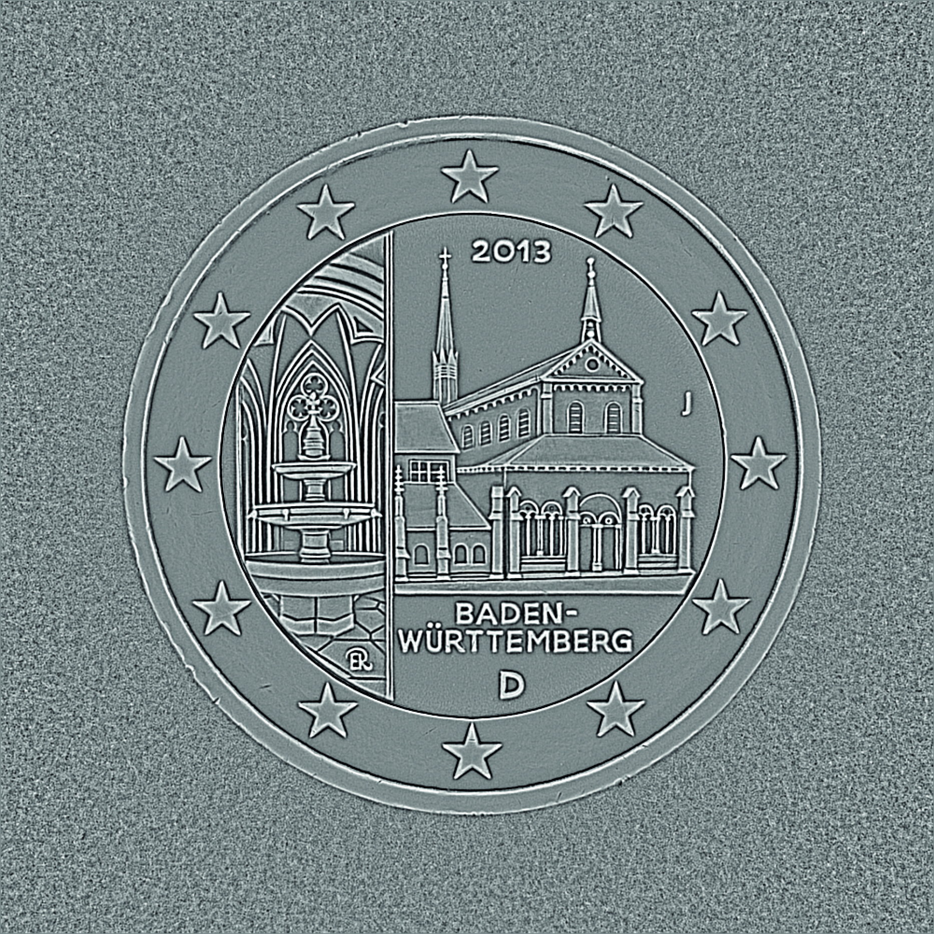
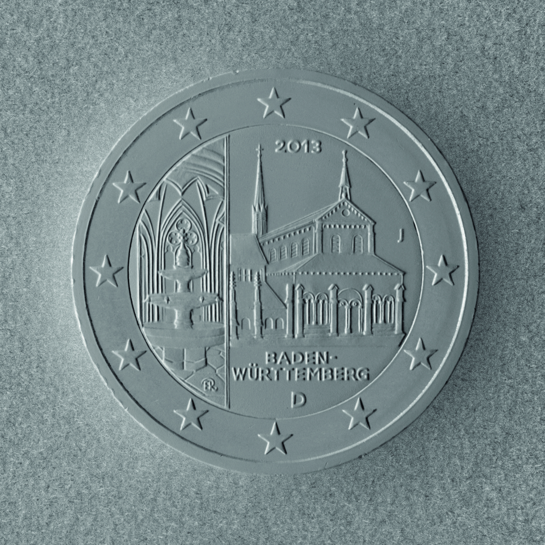
Fig. 2.10 Brightness.

System Message: WARNING/2 (/home/docs/checkouts/readthedocs.org/user_builds/fringes/checkouts/main/docs/source/02_tutorial/filter.rst, line 42)

Cannot scale image! Could not get size from "02_tutorial/filter/modulation.png": [Errno 2] No such file or directory: '02_tutorial/filter/modulation.png'

Fig. 2.11 Modulation.

System Message: WARNING/2 (/home/docs/checkouts/readthedocs.org/user_builds/fringes/checkouts/main/docs/source/02_tutorial/filter.rst, line 50)

Cannot scale image! Could not get size from "02_tutorial/filter/coordinate.png": [Errno 2] No such file or directory: '02_tutorial/filter/coordinate.png'

Fig. 2.12 Coordinate.

2.4.1. Direct and Global Illumination Component

The direct illumination component is just twice the measured modulation:

\(I_D = 2 \hat{b}\).

The global illumination component can be determined with

\(I_G = 2 (\hat{a} - \hat{b})\)

under the condition that the spatial frequency \(\nu\) is high enough [Nay06].

Both can be normalized into the range [0, 1) by dividing through the maximal possible gray value \(I_{max}\) of the recording camera.

"""Direct and global illumination component.

https://dl.acm.org/doi/abs/10.1145/1179352.1141977
"""

from fringes import Fringes
from fringes.filter import direct, indirect

f = Fringes()
f.v = 99, 100, 101  # spatial frequency 'v' must be high enough but still resolved by the recording camera

I = f.encode()
Irec = I  # todo: replace this line with recording data (cf. example in 'record.py')
a, b, x = f.decode(Irec)

d = direct(b)
g = indirect(a, b)

# show results
import matplotlib.pyplot as plt
from matplotlib import colors

fig, axs = plt.subplots(nrows=f.K, ncols=f.D)
fig.suptitle("global 'g'")
norm = colors.Normalize(vmin=g.min(), vmax=g.max())
images = []
for i_d in range(f.D):
    axs[0, i_d].set_title(f"{'yx'[f.axes[i_d]]}-direction")
    for i in range(f.K):
        if i_d == 0:
            axs[i, i_d].set_ylabel(f"{i}-th set")
        t = i_d * f.K + i
        images.append(axs[i, i_d].imshow(g[t, :, :, 0], norm=norm))  # shows only first color channel
fig.colorbar(images[0], ax=axs)

fig, axs = plt.subplots(nrows=f.K, ncols=f.D)
fig.suptitle("direct 'd'")
norm = colors.Normalize(vmin=d.min(), vmax=d.max())
images = []
for i_d in range(f.D):
    axs[0, i_d].set_title(f"{'yx'[f.axes[i_d]]}-direction")
    for i in range(f.K):
        if i_d == 0:
            axs[i, i_d].set_ylabel(f"{i}-th set")
        t = i_d * f.K + i
        images.append(axs[i, i_d].imshow(d[t, :, :, 0], norm=norm))  # shows only first color channel
fig.colorbar(images[0], ax=axs)

plt.show()

System Message: WARNING/2 (/home/docs/checkouts/readthedocs.org/user_builds/fringes/checkouts/main/docs/source/02_tutorial/filter.rst, line 77)

Cannot scale image! Could not get size from "02_tutorial/filter/direct.png": [Errno 2] No such file or directory: '02_tutorial/filter/direct.png'

Fig. 2.13 Direct illumination component.

System Message: WARNING/2 (/home/docs/checkouts/readthedocs.org/user_builds/fringes/checkouts/main/docs/source/02_tutorial/filter.rst, line 84)

Cannot scale image! Could not get size from "02_tutorial/filter/indirect.png": [Errno 2] No such file or directory: '02_tutorial/filter/indirect.png'

Fig. 2.14 Global illumination component.

2.4.2. Visibility and Exposure

In an alternative formulation, the absolute quantities offset \(a\) and amplitude \(b\) of the phase shifting equation are replaced by the maximal possible gray value \(I_{max}\), the relative quantities exposure \(E\) (relative average intensity) and visibility \(V\) (relative fringe contrast) [Fis12]:

\(I = a + b \cos(\varPhi) = I_{max} E [1 + V \cos(\varPhi)]\)

The two parameters \(E = \hat{a} / I_{max}\) and \(V = \hat{b_i} / \hat{a}\) describe the phase shifting signal \(I\) independently of the value range \([0, I_{max}]\) of the light source or camera. Both lie within the interval \([0, 1]\) with the additional condition \(E \le 1 / (1 + V)\); else, the radiance of the light source would be higher than the maximal possible value \(I_{max}\). Therefore, the valid values of \(V\) are limited for \(E > 0.5\). The optimal fringe contrast \(V = 1\) can be reached when \(E = 0.5\).

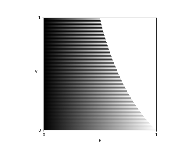
Fig. 2.15 Fringe pattern as a function of \(E\) and \(V\).

The advantage of this representation is the normalization of the descriptive parameters \(E\) and \(V\) and thereby the separation of additive and multiplicative influences.

The exposure \(E\) is affected by additional, constant light (not modulating the signal):

• the maximum brightness of the light source,

• the absorption of the sample

• the absorption of optical elements (e.g. filters),

• the exposure time and the aperture setting of the camera.

The visibility \(V\) is influenced by:

• the maximum contrast of the light source

• the surface quality of the sample (roughness, scattering),

• the position of the sample with regard to the focal plane of the lens (blurring due to defocus and depth of field),

• the camera lens’ modulation transfer function,

• the camera’s resolution (the camera pixel size projected onto the light source acts as a low pass filter).

"""Visibility and Exposure."""

from fringes import Fringes
from fringes.filter import exposure, visibility

f = Fringes()

I = f.encode()
Irec = I  # todo: replace this line with recording data (cf. example in 'record.py')
a, b, x = f.decode(Irec)

E = exposure(a, Irec)
V = visibility(a, b)

# show results
import matplotlib.pyplot as plt
from matplotlib import colors

fig, axs = plt.subplots(nrows=f.K, ncols=f.D, squeeze=False, num="visibility 'V'")
norm = colors.Normalize(vmin=V.min(), vmax=V.max())
for d in range(f.D):
    for i in range(f.K):
        if d == 0:
            axs[i, d].set_ylabel(f"{i}-th set")
        t = d * f.K + i
        image = axs[i, d].imshow(V[t, :, :, 0], norm=norm)  # shows only first color channel
fig.colorbar(image, ax=axs)

fig, axs = plt.subplots(ncols=f.D, squeeze=False, num="exposure 'E'")
norm = colors.Normalize(vmin=E.max(), vmax=E.max())
for d in range(f.D):
    axs[0, d].set_title(f"{'yx'[f.axes[d]]}-direction")
    image = axs[0, d].imshow(E[d, :, :, 0], norm=norm)  # shows only first color channel
fig.colorbar(image, ax=axs)

plt.show()

System Message: WARNING/2 (/home/docs/checkouts/readthedocs.org/user_builds/fringes/checkouts/main/docs/source/02_tutorial/filter.rst, line 140)

Cannot scale image! Could not get size from "02_tutorial/filter/visibility.png": [Errno 2] No such file or directory: '02_tutorial/filter/visibility.png'

Fig. 2.16 Visibility.

System Message: WARNING/2 (/home/docs/checkouts/readthedocs.org/user_builds/fringes/checkouts/main/docs/source/02_tutorial/filter.rst, line 147)

Cannot scale image! Could not get size from "02_tutorial/filter/exposure.png": [Errno 2] No such file or directory: '02_tutorial/filter/exposure.png'

Fig. 2.17 Exposure.

2.4.3. Verbose Results

Additionally to the already mentioned results brightness, modulation, coordinate, visibility and exposure, more intermediate and verbose results can be returned by setting the flag verbose in the method decode() to True:

"""Decode verbose results."""

from fringes import Fringes

f = Fringes()

I = f.encode()
Irec = I  # todo: replace this line with the recorded data (cf. example in 'record.py')
dec = f.decode(Irec, verbose=True)  # here, a namedtuple is returned (see usage below)

# show verbose results
import matplotlib.pyplot as plt
import numpy as np
from matplotlib import colors

fig, axs = plt.subplots(ncols=f.D, squeeze=False, num="uncertainty 'u'")
norm = colors.Normalize(vmin=dec.u.min(), vmax=dec.u.max())
for d in range(f.D):
    axs[0, d].set_title(f"{'yx'[f.axes[d]]}-direction")
    image = axs[0, d].imshow(dec.u[d, :, :, 0], norm=norm)  # shows only first color channel
fig.colorbar(image, ax=axs)

fig, axs = plt.subplots(ncols=f.D, squeeze=False, num="residuals 'r'")
norm = colors.Normalize(vmin=dec.r.max(), vmax=dec.r.max())
for d in range(f.D):
    axs[0, d].set_title(f"{'yx'[f.axes[d]]}-direction")
    image = axs[0, d].imshow(dec.r[d, :, :, 0], norm=norm)  # shows only first color channel
fig.colorbar(image, ax=axs)

fig, axs = plt.subplots(nrows=f.K, ncols=f.D, squeeze=False, num="fringe orders 'k'")
norm = colors.Normalize(vmin=dec.k.min(), vmax=dec.k.max())
for d in range(f.D):
    axs[0, d].set_title(f"{'yx'[f.axes[d]]}-direction")
    for i in range(f.K):
        if d == 0:
            axs[i, d].set_ylabel(f"{i}-th set")
        t = d * f.K + i
        image = axs[i, d].imshow(dec.k[t, :, :, 0], norm=norm)  # shows only first color channel
fig.colorbar(image, ax=axs)

fig, axs = plt.subplots(nrows=f.K, ncols=f.D, squeeze=False, num="phase 'p'")
norm = colors.Normalize(vmin=0, vmax=2 * np.pi)
for d in range(f.D):
    axs[0, d].set_title(f"{'yx'[f.axes[d]]}-direction")  # shows only first color channel
    for i in range(f.K):
        if d == 0:
            axs[i, d].set_ylabel(f"{i}-th set")
        t = d * f.K + i
        image = axs[i, d].imshow(dec.p[t, :, :, 0], norm=norm)
cbar = fig.colorbar(image, ax=axs, ticks=[0, np.pi, 2 * np.pi])
cbar.ax.set_yticklabels(["0", "$\\pi$", "$2\\pi$"])

plt.show()

The phase … after temporal demodulation … link to fundamentals

System Message: WARNING/2 (/home/docs/checkouts/readthedocs.org/user_builds/fringes/checkouts/main/docs/source/02_tutorial/filter.rst, line 167)

Cannot scale image! Could not get size from "02_tutorial/filter/phase.png": [Errno 2] No such file or directory: '02_tutorial/filter/phase.png'

Fig. 2.18 Phase.

---

The residuals … after optimization-based unwrapping … link to fundamentals

System Message: WARNING/2 (/home/docs/checkouts/readthedocs.org/user_builds/fringes/checkouts/main/docs/source/02_tutorial/filter.rst, line 190)

Cannot scale image! Could not get size from "02_tutorial/filter/residuals.png": [Errno 2] No such file or directory: '02_tutorial/filter/residuals.png'

Fig. 2.19 Residuals.

---

The uncertainty … after temporal demodulation i.e. unwrapping … best/minimal uncertainty if ui is set and correct fringe orders are found … link to fundamentals

System Message: WARNING/2 (/home/docs/checkouts/readthedocs.org/user_builds/fringes/checkouts/main/docs/source/02_tutorial/filter.rst, line 202)

Cannot scale image! Could not get size from "02_tutorial/filter/uncertainty.png": [Errno 2] No such file or directory: '02_tutorial/filter/uncertainty.png'

Fig. 2.20 Uncertainty.

2.4.4. Slope

If the deflectometric setup is calibrated, the slope of the surface can be computed from the coordinate.

“[Deflectometry] measures slopes (first order derivatives of the shape). The sensitivity to higher spatial frequencies is therefore amplified, resulting in excellent (sometimes excessive) sensitivity for small-scale irregularities and at the same time poor sensitivity and stability for low-order surface features.” [Bur23]

"""Slope."""

from fringes import Fringes

f = Fringes()

I = f.encode()
Irec = I  # todo: replace this line with the recorded data (cf. example in 'record.py')
a, b, x = f.decode(Irec)

s = x  # todo: compute slope from calibrated setup

# show results
import matplotlib.pyplot as plt
from matplotlib import colors

fig, axs = plt.subplots(ncols=f.D)
fig.suptitle("slope 's'")
norm = colors.Normalize(vmin=s.min(), vmax=s.max())
images = []
for d in range(f.D):
    axs[d].set_title(f"{'yx'[f.axes[d]]}-direction")
    images.append(axs[d].imshow(s[d, :, :, 0], norm=norm))  # shows only first color channel
fig.colorbar(images[0], ax=axs)
plt.show()

Fig. 2.21 Slope map in x-direction. Source: [SAC].

Fig. 2.22 Slope map in y-direction. Source: [SAC].

2.4.5. Curvature

“As an alternative use of [deflectometry] data, one may differentiate them and recover surface curvatures (combinations of second order shape derivatives […]. Unlike point positions and slopes, the latter are intrinsic local characteristics of the surface […] that are independent of its embedding in 3D space. As such, curvature maps are useful observables for various quality inspection tasks. Derivation of curvatures is less error-prone than shape integration and does not require accurate prior knowledge of the distance to the object.” [Bur23]

"""Curvature."""

from fringes import Fringes
from fringes.filter import curvature

f = Fringes()

I = f.encode()
Irec = I  # todo: replace this line with recording data (cf. example in 'record.py')
a, b, x = f.decode(Irec)

s = x  # todo: compute slope from calibrated setup
c = curvature(s)

# show result
import matplotlib.pyplot as plt

plt.figure("curvature 'c'")
plt.imshow(c[:, :, 0])  # only first color channel
plt.colorbar()
plt.show()

Fig. 2.23 Curvature map. Source: [SAC].

[Bur23] (1,2)

Burke et al., “Deflectometry for specular surfaces: an overview”, Advanced Optical Technologies, 2023.

[Fis12]

Fischer et al., “Vorhersage des Phasenrauschens in optischen Messsystemen mit strukturierter Beleuchtung”, Technisches Messen, 2012.

[Nay06]

Nayar et al., “Fast separation of direct and global components of a scene using high frequency illumination”, SIGGRAPH, 2006.

[SAC] (1,2,3)

SAC Sirius Advanced Cybernetics GmbH, “trevista”, product information sheet, 2018.